Encoding interactions

Interactions are always pairwise and always between encoders (and not features).

The supported interactions are between: (a) categorical and categorical encoders, (b) categorical and linear encoders, (c) categorical and spline encoders, (d) linear and linear encoders, and (e) spline and spline encoders.

All encoders have a n_features_out_ property after fitting.

import numpy as np
import pandas as pd
import matplotlib.pyplot as plt

from sklearn.datasets import make_friedman1
from sklearn.linear_model import LinearRegression
from sklearn.metrics import mean_squared_error
from sklearn.pipeline import Pipeline, FeatureUnion
from sklearn.model_selection import train_test_split

%matplotlib inline

from feature_encoders.utils import tensor_product, add_constant
from feature_encoders.generate import CyclicalFeatures, DatetimeFeatures
from feature_encoders.encode import (
    CategoricalEncoder,
    ICatEncoder,
    SplineEncoder,
    ISplineEncoder,
    IdentityEncoder,
    ProductEncoder,
    ICatLinearEncoder,
    ICatSplineEncoder
)

Load demo data

data = pd.read_csv('data/data.csv', parse_dates=[0], index_col=0)
data = data[~data['consumption_outlier']]

Pairwise interactions between categorical features

ICatEncoder encodes the interaction between two categorical features. Both encoders should have the same encode_as parameter.

If encode_as = 'onehot', it returns the tensor product of the results of the two encoders. The tensor product combines row-per-row the results from the first and the second encoder as follows:

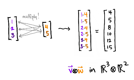
A small example of the tensor product function:

a = np.array([1, 10]).reshape(1, -1)
b = np.array([10, 20, 30]).reshape(1, -1)

tensor_product(a, b)

array([[ 10,  20,  30, 100, 200, 300]])

The easiest way to demonstate it is by combining hours of day and days of week into hours of week:

enc = DatetimeFeatures(subset=['dayofweek', 'hour', 'hourofweek'])
data = enc.fit_transform(data)

enc_dow = CategoricalEncoder(feature='dayofweek', encode_as='onehot')
feature_dow = enc_dow.fit_transform(data)
feature_dow.shape

(37287, 7)

enc_hour = CategoricalEncoder(feature='hour', encode_as='onehot')
feature_hour = enc_hour.fit_transform(data)
feature_hour.shape

(37287, 24)

enc = ICatEncoder(enc_dow, enc_hour).fit(data)
enc.n_features_out_

168

assert np.all(enc.transform(data).argmax(axis=1) == data['hourofweek'].values)

If encode_as = 'ordinal', it returns the combinations of the encoders’ results, where each combination is a string with : between the two values:

enc_dow = CategoricalEncoder(feature='dayofweek', encode_as='ordinal')
enc_hour = CategoricalEncoder(feature='hour', encode_as='ordinal')
enc = ICatEncoder(enc_dow, enc_hour)

feature_trf = enc.fit_transform(data)
feature_trf

array([['0:12'],
       ['0:12'],
       ['0:12'],
       ...,
       ['5:21'],
       ['5:21'],
       ['5:22']], dtype='<U13')

assert np.unique(feature_trf).size == 168

Pairwise interactions between numerical features

We can generate data for the “Friedman #1” regression problem:

\[y=10*sin(\pi*x_0*x_1) + 20*(x_2-0.5)^2 + 10*x_3+5 * x_4 + noise*N(0,1)\]

X, y = make_friedman1(n_samples=5000, n_features=5, noise=0.2)
X = pd.DataFrame(data=X, columns=[f'x_{i}' for i in range(5)])
y = pd.Series(data=y, index=X.index)
X.head()

	x_0	x_1	x_2	x_3	x_4
0	0.491884	0.597237	0.017681	0.753236	0.068667
1	0.281404	0.524407	0.769966	0.689059	0.385223
2	0.329995	0.170124	0.208075	0.390547	0.795747
3	0.772299	0.509458	0.309719	0.172743	0.203104
4	0.838131	0.057251	0.461958	0.006787	0.961568

X_train, X_test, y_train, y_test = train_test_split(X, y, test_size=0.5, shuffle=True)

enc_0 = SplineEncoder(feature='x_0',
                      n_knots=5,
                      degree=3,
                      strategy="quantile",
                      extrapolation="constant",
                      include_bias=True,
)

enc_1 = SplineEncoder(feature='x_1',
                      n_knots=5,
                      degree=3,
                      strategy="quantile",
                      extrapolation="constant",
                      include_bias=True,
)

enc_2 = SplineEncoder(feature='x_2',
                      n_knots=5,
                      degree=3,
                      strategy="quantile",
                      extrapolation="constant",
                      include_bias=True,
)

enc_3 = SplineEncoder(feature='x_3',
                      n_knots=5,
                      degree=3,
                      strategy="quantile",
                      extrapolation="constant",
                      include_bias=True,
)

enc_4 = SplineEncoder(feature='x_4',
                      n_knots=5,
                      degree=3,
                      strategy="quantile",
                      extrapolation="constant",
                      include_bias=True,
)

interact = ISplineEncoder(enc_0, enc_1)

pipeline = Pipeline([
    ('features', FeatureUnion([
                    ('inter', interact),
                    ('enc_2', enc_2),
                    ('enc_3', enc_3),
                    ('enc_4', enc_4)

                ])
    ),
    ('regression', LinearRegression(fit_intercept=False))
])

pipeline = pipeline.fit(X_train, y_train)

The root mean squared error is very close to the noise that was injected in the data (0.2):

print('Root mean squared out-of-sample error: '
      f'{mean_squared_error(np.array(y_test), pipeline.predict(X_test), squared=False)}'
)

Root mean squared out-of-sample error: 0.1980257834415656

Linear interations are also supported through ProductEncoder. ProductEncoder expects IdentityEncoders, which are utility encoders that return what they are fed.

enc_0 = IdentityEncoder(feature='x_0', include_bias=False,)
enc_1 = IdentityEncoder(feature='x_1', include_bias=False,)

interact = ProductEncoder(enc_0, enc_1)

This interaction is practically an element-wise multiplication of the two features:

assert np.all(interact.fit_transform(X).squeeze() == X[['x_0', 'x_1']].prod(axis=1))

Pairwise interactions between categorical and numerical features

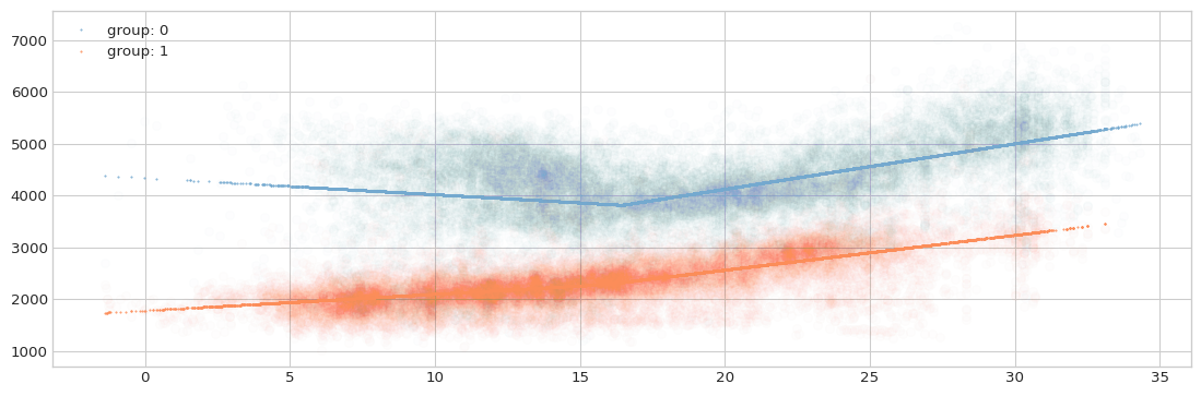
Suppose that we want to split the hours of the week in the demo data into two distinct categories (according to the similarities of the consumption data) and then model the impact of the outdoor temperature during each one of these categories: consumption ~ temperature:hour_of_week.

First, we can explore the case where we split all the data by the reduced hour_of_week and fit a consumption ~ temperature model to each group:

enc_occ = CategoricalEncoder(
            feature='hourofweek',
            max_n_categories=2,
            stratify_by='temperature',
            min_samples_leaf=15,
            encode_as='ordinal'
)

X = data[['hourofweek', 'temperature']]
y = data['consumption']

data['groups'] = enc_occ.fit_transform(X, y)

models = {}

for group, grouped_data in data.groupby('groups'):
    model = LinearRegression(fit_intercept=True).fit(grouped_data[['temperature']],
                                                     grouped_data['consumption'])
    models[group] = model

color_list = ['#74a9cf', '#fc8d59']

with plt.style.context('seaborn-whitegrid'):
    fig = plt.figure(figsize=(14, 4.5), dpi=96)
    layout = (1, 1)
    ax = plt.subplot2grid(layout, (0, 0))

    resid = []
    for i, (group, grouped_data) in enumerate(data.groupby('groups')):
        pred = models[group].predict(grouped_data[['temperature']])
        resid.append(grouped_data['consumption'].values - pred)

        ax.plot(grouped_data['temperature'], pred,
                label=f'group: {group}', c=color_list[i])
        ax.plot(grouped_data['temperature'], grouped_data['consumption'],
                'o', c=color_list[i], alpha=0.01)

    ax.legend(loc='upper left')

print(f'Mean squared error: {np.mean(np.concatenate(resid)**2)}')

Mean squared error: 351555.77145852696

The same result can be achieved by first encoding the hour_of_week feature in one-hot form and then taking the tensor product between its encoding and the temperature feature. In this case, an intercept must be added directly to the temperature feature, so that it is possible to model a different intercept for each categorical feature’s level:

enc_occ = CategoricalEncoder(
            feature='hourofweek',
            max_n_categories=2,
            stratify_by='temperature',
            min_samples_leaf=15,
            encode_as='onehot'
)
feature_cat = enc_occ.fit_transform(X, y)

features = tensor_product(feature_cat, add_constant(X['temperature']))

model = LinearRegression(fit_intercept=False).fit(features, y)
pred = model.predict(features)

resid = y.values - pred
print(f'Mean squared error: {np.mean(resid**2)}')

Mean squared error: 351555.771458527

color_list = ['#74a9cf', '#fc8d59']

with plt.style.context('seaborn-whitegrid'):
    fig = plt.figure(figsize=(14, 4.5), dpi=96)
    layout = (1, 1)
    ax = plt.subplot2grid(layout, (0, 0))

    for i in range(enc_occ.n_features_out_):
        mask = feature_cat[:, i]==1
        ax.plot(data['temperature'][mask], pred[mask], label=f'group: {i}',
                c=color_list[i])
        ax.plot(data['temperature'][mask], data['consumption'][mask], 'o',
                c=color_list[i], alpha=0.01)

    ax.legend(loc='upper left')

The conclusion here is that for the case of one categorical and one linear numerical feature, we can model the interaction by first encoding the categorical feature in one-hot form and then taking the tensor product between this encoding and the numerical feature.

This is supported by ICatLinearEncoder:

enc_occ = CategoricalEncoder(
            feature='hourofweek',
            max_n_categories=2,
            stratify_by='temperature',
            min_samples_leaf=15,
            encode_as='onehot'
)
enc_num = IdentityEncoder(feature='temperature', include_bias=True)

enc = ICatLinearEncoder(encoder_cat=enc_occ, encoder_num=enc_num)

features = enc.fit_transform(X, y)
model = LinearRegression(fit_intercept=False).fit(features, y)
pred = model.predict(features)

resid = y.values - pred
print(f'Mean squared error: {np.mean(resid**2)}')

Mean squared error: 351555.77145852696

Next, we want to encode the temperature feature with splines so that to capture potential non-linearities.

A *first split, then encode* strategy looks like this:

models = {}
encoders = {}

for group, grouped_data in data.groupby('groups'):
    enc = SplineEncoder(feature='temperature',
                        n_knots=3,
                        degree=1,
                        strategy='uniform',
                        extrapolation='constant',
                        include_bias=True,
    )
    features = enc.fit_transform(grouped_data)
    model = LinearRegression(fit_intercept=False).fit(features, grouped_data['consumption'])
    models[group] = model
    encoders[group] = enc

color_list = ['#74a9cf', '#fc8d59']

with plt.style.context('seaborn-whitegrid'):
    fig = plt.figure(figsize=(14, 4.5), dpi=96)
    layout = (1, 1)
    ax = plt.subplot2grid(layout, (0, 0))

    resid = []
    for i, (group, grouped_data) in enumerate(data.groupby('groups')):
        features = encoders[group].transform(grouped_data)
        pred = models[group].predict(features)
        resid.append(grouped_data['consumption'].values - pred)

        ax.plot(grouped_data['temperature'], pred, '.', ms=1,
                label=f'group: {group}', c=color_list[i])
        ax.plot(grouped_data['temperature'], grouped_data['consumption'],
                'o', c=color_list[i], alpha=0.01)

    ax.legend(loc='upper left')

print(f'Mean squared error: {np.mean(np.concatenate(resid)**2)}')

Mean squared error: 329833.6746798132

This first split, then encode strategy is implemented by ICatSplineEncoder. Note that:

• If the categorical encoder is already fitted, it will not be re-fitted during fit or fit_transform.

• The numerical encoder will always be fitted (one encoder per level of categorical feature).

Since we employ cardinality reduction, the categorical encoder should be fitted using all data.

enc_occ = CategoricalEncoder(
            feature='hourofweek',
            max_n_categories=2,
            stratify_by='temperature',
            min_samples_leaf=15,
            encode_as='onehot'
        )

# Fit the categorical encoder at global level
enc_occ = enc_occ.fit(X, y)

enc_num = SplineEncoder(feature='temperature',
                        n_knots=3,
                        degree=1,
                        strategy='uniform',
                        extrapolation='constant',
                        include_bias=True,
          )

enc = ICatSplineEncoder(encoder_cat=enc_occ, encoder_num=enc_num)
features = enc.fit_transform(X)
model = LinearRegression(fit_intercept=False).fit(features, y)
pred = model.predict(features)

resid = y.values - pred
print(f'Mean squared error: {np.mean(resid**2)}')

Mean squared error: 329833.6746798132

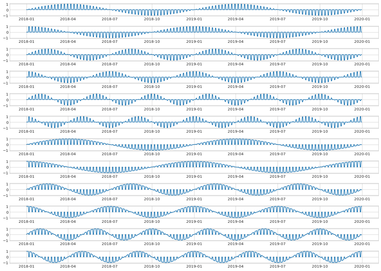
Conditional seasonality

By combining a CategoricalEncoder with a CyclicalFeatures generator, we can create features of conditional seasonalities very similarly to how the Prophet library does it:

https://facebook.github.io/prophet/docs/seasonality,_holiday_effects,_and_regressors.html#seasonalities-that-depend-on-other-factors

data = pd.DataFrame(index=pd.date_range(start='1/1/2018', end='31/12/2019', freq='D'))
data['weekday'] = data.index.dayofweek < 5

data.head()

	weekday
2018-01-01	True
2018-01-02	True
2018-01-03	True
2018-01-04	True
2018-01-05	True

data = CyclicalFeatures(seasonality='yearly', fourier_order=3).fit_transform(data)
data.head()

	weekday	yearly_delim_0	yearly_delim_1	yearly_delim_2	yearly_delim_3	yearly_delim_4	yearly_delim_5
2018-01-01	True	0.008601	0.999963	0.017202	0.999852	0.025801	0.999667
2018-01-02	True	0.025801	0.999667	0.051584	0.998669	0.077334	0.997005
2018-01-03	True	0.042993	0.999075	0.085906	0.996303	0.128661	0.991689
2018-01-04	True	0.060172	0.998188	0.120126	0.992759	0.179645	0.983732
2018-01-05	True	0.077334	0.997005	0.154204	0.988039	0.230151	0.973155

enc_cat = CategoricalEncoder(feature='weekday', encode_as='onehot')
features_cat = enc_cat.fit_transform(data)
features_cat.shape

(730, 2)

enc_lin = IdentityEncoder(feature='yearly', as_filter=True)
features_cyc = enc_lin.fit_transform(data)
features_cyc.shape

(730, 6)

As tensor product:

features_tp = tensor_product(features_cat, features_cyc)
features_tp = pd.DataFrame(data=features_tp, index=data.index)
features_tp.shape

(730, 12)

with plt.style.context('seaborn-whitegrid'):
    fig, axs = plt.subplots(features_tp.shape[1], figsize=(14, 10), dpi=96)

    for i in range(features_tp.shape[1]):
        axs[i].plot(features_tp.loc[:, i])

fig.tight_layout()

assert np.all(features_tp.loc[data['weekday'], [0, 1, 2, 3, 4, 5]] == 0)
assert np.all(features_tp.loc[~data['weekday'], [6, 7, 8, 9, 10, 11]] == 0)

The same thing can be achieved by:

enc_cat = CategoricalEncoder(feature='weekday', encode_as='onehot')
enc_num = IdentityEncoder(feature='yearly', as_filter=True)

enc = ICatLinearEncoder(encoder_cat=enc_cat, encoder_num=enc_num)
features_enc = enc.fit_transform(data)
features_enc = pd.DataFrame(data=features_enc, index=data.index)

assert np.all(features_tp == features_enc)

Note that for the case of cyclical data, a first split then encode and a first encode then split strategies are equivalent, because the encoding uses only the information of each row and not any other value from the same column.

---