The functionality for generating new features

The feature-encoders library includes a few feature generators:

• TrendFeatures: Generates time trend features.

• DatetimeFeatures: Generates date and time features (such as the month of the year or the hour of the week).

• CyclicalFeatures: Creates cyclical (seasonal) features as Fourier terms (similarly to the way the Prophet library generates seasonality features).

All feature generators generate pandas DataFrames, and they all have two common parameters:

remainder : str, {'drop', 'passthrough'}, default='passthrough'
    By specifying `remainder='passthrough'`, all the remaining columns of the
    input dataset will be automatically passed through (concatenated with the
    output of the transformer).
replace : bool, default=False
    Specifies whether replacing an existing column with the same name is allowed
    (when `remainder=passthrough`).

import pandas as pd
import matplotlib.pyplot as plt

from sklearn.linear_model import LinearRegression

%matplotlib inline

from feature_encoders.generate import CyclicalFeatures, DatetimeFeatures, TrendFeatures

Load demo data

data = pd.read_csv('data/data.csv', parse_dates=[0], index_col=0)
data = data[~data['consumption_outlier']]

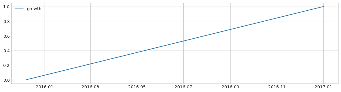
Create time trend features

The ds argument corresponds to the name of the input dataframe’s column that contains datetime information. If None, it is assumed that the datetime information is provided by the input dataframe’s index.

enc = TrendFeatures(ds=None, name='growth', remainder='drop')
features = enc.fit_transform(data)

with plt.style.context('seaborn-whitegrid'):
    fig = plt.figure(figsize=(14, 3.54), dpi=96)
    layout = (1, 1)
    ax = plt.subplot2grid(layout, (0, 0))

    ax.plot(features['growth'], label='growth')
    ax.legend(loc='upper left')

Add date and time features

The subset argument corresponds to the names of the features to generate. If None, all features will be produced: ‘month’, ‘week’, ‘dayofyear’, ‘dayofweek’, ‘hour’, ‘hourofweek’. The last 2 features are generated only if the timestep of the input’s feature (or index if feature is None) is smaller than pandas.Timedelta(days=1).

enc = DatetimeFeatures(ds=None, subset=None, remainder='drop')
features = enc.fit_transform(data)
features.columns

Index(['month', 'week', 'dayofyear', 'dayofweek', 'hour', 'hourofweek'], dtype='object')

enc = DatetimeFeatures(ds=None, remainder='drop', subset=['month', 'hourofweek'])
features = enc.fit_transform(data)
features.columns

Index(['month', 'hourofweek'], dtype='object')

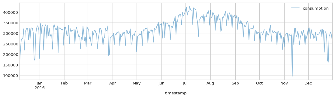
Encode cyclical (seasonal) features

The encoder is parameterized by period (number of days in one period) and fourier_order (number of Fourier components to use).

It can provide default values for period and fourier_order if seasonality is one of daily, weekly or yearly.

daily_consumption = data[['consumption']].resample('D').sum()

with plt.style.context('seaborn-whitegrid'):
    fig = plt.figure(figsize=(14, 3.54), dpi=96)
    layout = (1, 1)
    ax = plt.subplot2grid(layout, (0, 0))

    daily_consumption.plot(ax=ax, alpha=0.5)

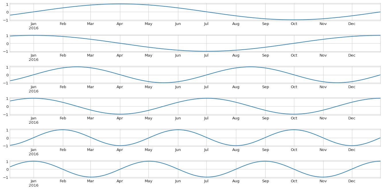
The number of seasonality features is always twice the fourier_order.

enc = CyclicalFeatures(ds=None, seasonality='yearly', fourier_order=3, remainder='drop')
features = enc.fit_transform(daily_consumption)
features.columns

Index(['yearly_delim_0', 'yearly_delim_1', 'yearly_delim_2', 'yearly_delim_3',
       'yearly_delim_4', 'yearly_delim_5'],
      dtype='object')

Now let’s plot the new features:

with plt.style.context('seaborn-whitegrid'):
    fig, axs = plt.subplots(2*enc.fourier_order, figsize=(14, 7), dpi=96)

    for i, col in enumerate(features.columns):
        features[col].plot(ax=axs[i])
        axs[i].set_xlabel(None)

fig.tight_layout()

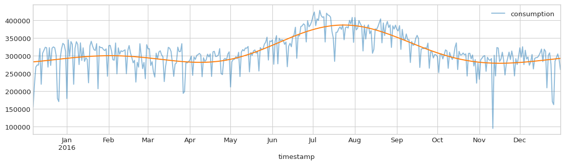
Let’s also see how well this transformation works:

regr = LinearRegression(fit_intercept=True).fit(features, daily_consumption)
pred = regr.predict(features)

with plt.style.context('seaborn-whitegrid'):
    fig = plt.figure(figsize=(14, 3.54), dpi=96)
    layout = (1, 1)
    ax = plt.subplot2grid(layout, (0, 0))

    daily_consumption.plot(ax=ax, alpha=0.5)
    pd.Series(pred.squeeze(), index=daily_consumption.index).plot(ax=ax)

---