Applications of feature-encoders

In this section, we present two applications:

• one for a simple linear regression model, and

• one for a grouped linear regression model (a model that construct one estimator per data group, splits data by values of a single column and fits one estimator per group).

import json
import numpy as np
import pandas as pd
import matplotlib.pyplot as plt

from sklearn.cluster import KMeans
from sklearn.linear_model import LinearRegression

%matplotlib inline

from feature_encoders.utils import load_config
from feature_encoders.generate import DatetimeFeatures
from feature_encoders.encode import CategoricalEncoder, SplineEncoder, ICatSplineEncoder
from feature_encoders.compose import ModelStructure
from feature_encoders.models import LinearPredictor, GroupedPredictor

def cvrmse(y_true, y_pred):
    resid = y_true - y_pred
    return float(np.sqrt((resid ** 2).sum() / len(resid)) / np.mean(y_true))


def nmbe(y_true, y_pred):
    resid = y_true - y_pred
    return float(np.mean(resid) / np.mean(y_true))

Load demo data

The data consists of the energy consumption of a building and the outdoor air temperature.

data = pd.read_csv('data/data.csv', parse_dates=[0], index_col=0)
data = data[~data['consumption_outlier']]

X = data[['temperature']]
y = data['consumption']

Linear regression model

The simplest model to use is a model that includes only the hour of the week as a feature. The hour of the week is a categorical feature and it can be encoded in one-hot form:

features = DatetimeFeatures(subset='hourofweek', remainder='drop').fit_transform(X)
dmatrix = CategoricalEncoder(feature='hourofweek', encode_as='onehot').fit_transform(features)

We can fit a linear model:

model = LinearRegression(fit_intercept=False).fit(dmatrix, y)

… and evaluate it in-sample:

pred = model.predict(dmatrix)

y_true = y.values

print(f"In-sample CV(RMSE) (%): {cvrmse(y_true, pred)*100}")
print(f"In-sample NMBE (%): {nmbe(y_true, pred)*100}")

In-sample CV(RMSE) (%): 19.332298975680697
In-sample NMBE (%): 7.804127359819421e-15

The degrees of freedom of the model are:

np.linalg.matrix_rank(dmatrix)

168

The impact of the hour of the week on energy consumption is then:

pred = pd.DataFrame(data=pred, index=y.index, columns=['hourofweek_impact'])

date_enc = DatetimeFeatures(remainder='passthrough', subset='hourofweek')
to_plot = date_enc.fit_transform(pred).groupby('hourofweek').mean()


colors = ['#8c510a', '#d8b365', '#f6e8c3', '#f5f5f5', '#c7eae5', '#5ab4ac', '#01665e']

with plt.style.context('seaborn-whitegrid'):
    fig = plt.figure(figsize=(12, 3), dpi=96)
    layout = (1, 1)
    ax = plt.subplot2grid(layout, (0, 0))

    intervals = np.split(to_plot.index, 7)
    for i, item in enumerate(intervals):
        ax.axvspan(item[0], item[-1], alpha=0.3, color=colors[i])

    to_plot.plot(ax=ax)
    ax.set_xlabel('Hour of week')
    ax.legend(['Average contribution of hour-of-week feature'], fancybox=True, frameon=True)

We can reduce the number of categories for the hour-of-week feature while retaining as much as possible the feature’s predictive capability:

features = DatetimeFeatures(subset='hourofweek', remainder='drop').fit_transform(X)
enc = CategoricalEncoder(feature='hourofweek', encode_as='onehot', max_n_categories=60)
dmatrix = enc.fit_transform(features, y)

model = LinearRegression(fit_intercept=False).fit(dmatrix, y)
pred = model.predict(dmatrix)

print(f"In-sample CV(RMSE) (%): {cvrmse(y_true, pred)*100}")
print(f"In-sample NMBE (%): {nmbe(y_true, pred)*100}")

In-sample CV(RMSE) (%): 19.34946719265366
In-sample NMBE (%): 4.263718362437927e-14

This is practically the same performance with one third of the degrees of freedom:

np.linalg.matrix_rank(dmatrix)

60

Another component to include in the model is an interaction term between the hour of the week and the temperature.

The TOWT model estimates the temperature effect separately for periods of the day with high and with low energy consumption in order to distinguish between occupied and unoccupied building periods.

To this end, a flexible curve is fitted on the consumption~temperature relationship, and if more than the 65% of the data points that correspond to a specific time-of-week are above the fitted curve, the corresponding hour is flagged as “Occupied”, otherwise it is flagged as “Unoccupied.”

We can apply this approach using feature-encoders functionality:

enc = SplineEncoder(feature='temperature', degree=1, strategy='uniform').fit(X)
dmatrix = enc.transform(X)

model = LinearRegression(fit_intercept=False).fit(dmatrix, y)
pred = model.predict(dmatrix)
pred = pd.Series(data=pred, index=y.index)

with plt.style.context('seaborn-whitegrid'):
    fig = plt.figure(figsize=(12, 3), dpi=96)
    layout = (1, 1)
    ax = plt.subplot2grid(layout, (0, 0))

    ax.scatter(X['temperature'], y, s=1, alpha=0.2)

    X_sorted = X.sort_values(by='temperature')
    ax.plot(X_sorted, pred.loc[X_sorted.index], c='#cc4c02')

resid = y - pred
mask = resid > 0
mask = DatetimeFeatures(subset='hourofweek').fit_transform(mask.to_frame('freq'))
occupied = mask.groupby('hourofweek')['freq'].mean() > 0.65
occupied = occupied.to_dict()

features = DatetimeFeatures(subset='hourofweek').fit_transform(X)
features['occupied'] = features['hourofweek'].map(lambda x: occupied[x])
features.head()

	temperature	hourofweek	occupied
timestamp
2015-12-07 12:00:00	14.300	12	True
2015-12-07 12:15:00	14.525	12	True
2015-12-07 12:30:00	14.750	12	True
2015-12-07 12:45:00	14.975	12	True
2015-12-07 13:00:00	15.200	13	True

enc_temp = SplineEncoder(feature='temperature', degree=1, strategy='uniform')
enc_occ = CategoricalEncoder(feature='occupied', encode_as='onehot')
enc_occ = enc_occ.fit(features) #fit before passed to the interaction

enc = ICatSplineEncoder(encoder_cat=enc_occ, encoder_num=enc_temp)
dmatrix = enc.fit_transform(features)

model = LinearRegression(fit_intercept=False).fit(dmatrix, y)
pred = model.predict(dmatrix)

print(f"In-sample CV(RMSE) (%): {cvrmse(y_true, pred)*100}")
print(f"In-sample NMBE (%): {nmbe(y_true, pred)*100}")

In-sample CV(RMSE) (%): 18.2731614241806
In-sample NMBE (%): 2.152083291755081e-14

np.linalg.matrix_rank(dmatrix)

10

Alternatively, we can rely on feature-encoders functionality to categorize the hours of the week into the two most dissimilar categories in terms of energy consumption given temperature information:

features = DatetimeFeatures(subset='hourofweek').fit_transform(X)

enc_temp = SplineEncoder(feature='temperature',
                         degree=1,
                         strategy='uniform'
)
enc_occ = CategoricalEncoder(feature='hourofweek',
                             max_n_categories=2,
                             stratify_by='temperature',
                             min_samples_leaf=15
)
enc_occ = enc_occ.fit(features, y) #fit before passed to the interaction

enc = ICatSplineEncoder(encoder_cat=enc_occ, encoder_num=enc_temp)
dmatrix = enc.fit_transform(features)

model = LinearRegression(fit_intercept=False).fit(dmatrix, y)
pred = model.predict(dmatrix)

print(f"In-sample CV(RMSE) (%): {cvrmse(y_true, pred)*100}")
print(f"In-sample NMBE (%): {nmbe(y_true, pred)*100}")

In-sample CV(RMSE) (%): 17.4373587893191
In-sample NMBE (%): 8.789160508284433e-14

The prediction results are better while the number of the degrees of freedom is the same:

np.linalg.matrix_rank(dmatrix)

10

Then, the consumption~temperature curves per category of hour of week are:

date_enc = DatetimeFeatures(remainder='passthrough', subset='hourofweek')

intervals = pd.concat(
    ( pd.cut(X['temperature'], 15, precision=0),
      pd.DataFrame(data=pred, index=X.index, columns=['temperature_impact'])
    ),
    axis=1
)

enc_cat = enc_occ.feature_pipeline_['reduce_dimension']
intervals = date_enc.fit_transform(intervals)
intervals['hourofweek'] = intervals['hourofweek'].map(lambda x: enc_cat.mapping_[x])

to_plot = (
    intervals.groupby(['hourofweek', 'temperature'])['temperature_impact']
             .mean()
             .unstack()
)

colors = ['#8c510a', '#df65b0']

with plt.style.context('seaborn-whitegrid'):
    fig = plt.figure(figsize=(12, 3), dpi=96)
    layout = (1, 1)
    ax = plt.subplot2grid(layout, (0, 0))

    for i, (idx, values) in enumerate(to_plot.iterrows()):
        values.plot(ax=ax, lw=2, alpha=0.6, label=f'category {idx}', color=colors[i])

    ax.xaxis.set_major_locator(plt.MaxNLocator(10))
    ax.set_xlabel('Temperature intervals')
    ax.legend(fancybox=True, frameon=True)

In confing/models, there is a YAML file (towt.yaml) that defines a linear regression model with the two components above and two additional ones:

1. A categorical feature for the different months in the dataset.

2. A linear term for the temperature as a main effect. The interaction term between temperature and the hour of the week “corrects” the predictions of the temperature’s linear term in the main effects.

model_conf, feature_conf = load_config(model='towt', features='default')

print(json.dumps(model_conf, indent=4))

{
    "add_features": {
        "time": {
            "type": "datetime",
            "subset": "month, hourofweek"
        }
    },
    "regressors": {
        "month": {
            "feature": "month",
            "type": "categorical",
            "encode_as": "onehot"
        },
        "tow": {
            "feature": "hourofweek",
            "type": "categorical",
            "max_n_categories": 60,
            "encode_as": "onehot"
        },
        "lin_temperature": {
            "feature": "temperature",
            "type": "linear"
        },
        "flex_temperature": {
            "feature": "temperature",
            "type": "spline",
            "n_knots": 5,
            "degree": 1,
            "strategy": "uniform",
            "extrapolation": "constant",
            "include_bias": true,
            "interaction_only": true
        }
    },
    "interactions": {
        "tow, flex_temperature": {
            "tow": {
                "max_n_categories": 2,
                "stratify_by": "temperature",
                "min_samples_leaf": 15
            }
        }
    }
}

The feature_encoders.models.LinearPredictor is a linear/ridge regression model that can be created using model configurations such as the above.

model_structure = ModelStructure.from_config(model_conf, feature_conf)
model = LinearPredictor(model_structure=model_structure)

Fit with available data:

%%time
model = model.fit(X, y)

Wall time: 2.4 s

Evaluate the model in-sample:

%%time
pred = model.predict(X)

print(f"In-sample CV(RMSE) (%): {cvrmse(y, pred['consumption'])*100}")
print(f"In-sample NMBE (%): {nmbe(y, pred['consumption'])*100}")

In-sample CV(RMSE) (%): 15.718435024677973
In-sample NMBE (%): 6.953335826993842e-05
Wall time: 290 ms

The effective number of parameters (i.e. the degrees of freedom) is:

model.dof

79

This is how the design matrix of the regression corresponds to each regressor:

model.composer_.component_matrix

component	lin_temperature	month	tow	tow:flex_temperature
col
0	0	1	0	0
1	0	1	0	0
2	0	1	0	0
3	0	1	0	0
4	0	1	0	0
...	...	...	...	...
78	0	0	0	1
79	0	0	0	1
80	0	0	0	1
81	0	0	0	1
82	0	0	0	1

83 rows × 4 columns

This makes it easy to decompose the prediction into components (the regularization term alpha=0.01 in the LinearPredictor was used primarily so that the individual components have reasonable values):

%%time
pred = model.predict(X, include_components=True)
pred.head()

Wall time: 337 ms

	consumption	lin_temperature	month	tow	tow:flex_temperature
timestamp
2015-12-07 12:00:00	4087.304937	1569.095673	593.424166	402.220121	1522.564976
2015-12-07 12:15:00	4084.172916	1593.784242	593.424166	402.220121	1494.744387
2015-12-07 12:30:00	4081.040895	1618.472810	593.424166	402.220121	1466.923798
2015-12-07 12:45:00	4077.908875	1643.161378	593.424166	402.220121	1439.103209
2015-12-07 13:00:00	4144.719000	1667.849947	593.424166	472.162267	1411.282620

assert np.allclose(pred['consumption'],
            pred[[col for col in pred.columns if col != 'consumption']].sum(axis=1)
)

with plt.style.context('seaborn-whitegrid'):
    fig = plt.figure(figsize=(12, 3), dpi=96)
    layout = (1, 1)
    ax = plt.subplot2grid(layout, (0, 0))

    pred['consumption'][:1344].plot(ax=ax, alpha=0.8) #2 weeks data
    y[:1344].plot(ax=ax, alpha=0.5)

Grouped linear regression model

The feature_encoders.models.GroupedPredictor can be applied on different clusters of a dataset. For this example, we assume that the clusters are created by a KMeans approach that is applied on daily consumption profiles, but there are smarter methods to distinguish between consumption profiles while ensuring that they are reliable during prediction (when no consumption data is available - see for instance how the eensight tool for automated M&V approaches this problem).

Since each of the models in the ensemble predicts on a different subset of the input data (an observation cannot belong to more than one clusters), the final prediction is generated by vertically concatenating all the individual models’ predictions.

data['time'] = data.index.time
data['date'] = data.index.date

to_cluster = data.pivot(index='date', columns='time', values='consumption')
to_cluster = to_cluster.fillna(method='bfill').fillna(method='ffill')

kmeans = KMeans(n_clusters=3).fit(to_cluster.values)
groups = pd.Series(data=kmeans.labels_, index=to_cluster.index)
data['group'] = data['date'].map(lambda x: str(groups[x]))

colors = ['#8c510a', '#3690c0', '#dd3497']

with plt.style.context('seaborn-whitegrid'):
    fig = plt.figure(figsize=(12, 3), dpi=96)
    layout = (1, 1)
    ax = plt.subplot2grid(layout, (0, 0))

    for i, (_, grouped) in enumerate(data.groupby('group')):
        grouped.pivot(index='time', columns='date', values='consumption').plot(
            ax=ax, legend=False, alpha=0.05, color=colors[i])

X = data[['temperature', 'group']]
y = data['consumption']

model = GroupedPredictor(
            group_feature='group',
            model_conf=model_conf,
            feature_conf=feature_conf
)

%%time
model = model.fit(X, y)

Wall time: 2.83 s

The GroupedPredictor applies the feature generation transformers defined in model_conf directly on the dataset before it is split per cluster:

model.added_features_

[DatetimeFeatures(subset=['month', 'hourofweek'])]

… whereas the cluster predictors do not see or apply any feature generator:

for group, est in model.estimators_.items():
    print(group, '-->', est.composer_.added_features_)

0 --> []
1 --> []
2 --> []

In addition, GroupedPredictor fits all categorical encoders in ordinal form, and then passes the encoded data to each cluster predictor:

for name, encoder in model.encoders_['main_effects'].items():
    print(name, '-->', encoder)

month --> CategoricalEncoder(encode_as='ordinal', feature='month')
tow --> CategoricalEncoder(encode_as='ordinal', feature='hourofweek',
                   max_n_categories=60)

… and adds the cluster feature in every stratify_by that is not empty:

for pair_name, encoder in model.encoders_['interactions'].items():
    print(pair_name, '-->', encoder)

('tow', 'flex_temperature') --> {'tow': CategoricalEncoder(encode_as='ordinal', feature='hourofweek',
                   max_n_categories=2, min_samples_leaf=15,
                   stratify_by=['group', 'temperature'])}

The cluster predictors get encoders that operate on data that has been transformed by the categorical encoders of the GroupedPredictor. In this way, categorical data is always encoded with full information (while numerical data is encoded at the cluster level):

for group, est in model.estimators_.items():
    print('group ', group)
    for name, encoder in est.composer_.encoders_['main_effects'].items():
        print(name, '-->', encoder)
    print('\n')

group  0
month --> CategoricalEncoder(feature='month__for__month')
tow --> CategoricalEncoder(feature='hourofweek__for__tow')
lin_temperature --> IdentityEncoder(feature='temperature')


group  1
month --> CategoricalEncoder(feature='month__for__month')
tow --> CategoricalEncoder(feature='hourofweek__for__tow')
lin_temperature --> IdentityEncoder(feature='temperature')


group  2
month --> CategoricalEncoder(feature='month__for__month')
tow --> CategoricalEncoder(feature='hourofweek__for__tow')
lin_temperature --> IdentityEncoder(feature='temperature')

for group, est in model.estimators_.items():
    print('group ', group)
    for name, encoder in est.composer_.encoders_['interactions'].items():
        print(name, '-->', encoder)
    print('\n')

group  0
('tow', 'flex_temperature') --> ICatSplineEncoder(encoder_cat=CategoricalEncoder(feature='hourofweek__for__tow:flex_temperature',
                                                 min_samples_leaf=15),
                  encoder_num=SplineEncoder(degree=1, feature='temperature'))


group  1
('tow', 'flex_temperature') --> ICatSplineEncoder(encoder_cat=CategoricalEncoder(feature='hourofweek__for__tow:flex_temperature',
                                                 min_samples_leaf=15),
                  encoder_num=SplineEncoder(degree=1, feature='temperature'))


group  2
('tow', 'flex_temperature') --> ICatSplineEncoder(encoder_cat=CategoricalEncoder(feature='hourofweek__for__tow:flex_temperature',
                                                 min_samples_leaf=15),
                  encoder_num=SplineEncoder(degree=1, feature='temperature'))

%%time
pred = model.predict(X)

print(f"In-sample CV(RMSE) (%): {cvrmse(y, pred['consumption'])*100}")
print(f"In-sample NMBE (%): {nmbe(y, pred['consumption'])*100}")

In-sample CV(RMSE) (%): 13.537423014233884
In-sample NMBE (%): 0.0001238626531768618
Wall time: 567 ms

The number of parameters is:

model.n_parameters

242

the degrees of freedom:

model.dof

230

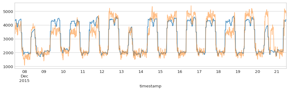
Since we have fitted one LinearPredictor per cluster, it is still easy to decompose the prediction into components:

%%time
pred = model.predict(X, include_components=True)
pred.head()

Wall time: 650 ms

	consumption	lin_temperature	month	tow	tow:flex_temperature
timestamp
2015-12-07 12:00:00	4323.340119	1439.591296	669.917419	535.061043	1678.770360
2015-12-07 12:15:00	4315.882619	1462.242208	669.917419	535.061043	1648.661948
2015-12-07 12:30:00	4308.425119	1484.893120	669.917419	535.061043	1618.553536
2015-12-07 12:45:00	4305.942539	1507.544032	669.917419	535.061043	1593.420044
2015-12-07 13:00:00	4398.279232	1530.194944	669.917419	629.880316	1568.286553

assert np.allclose(pred['consumption'],
            pred[[col for col in pred.columns if col != 'consumption']].sum(axis=1)
)

with plt.style.context('seaborn-whitegrid'):
    fig = plt.figure(figsize=(12, 3), dpi=96)
    layout = (1, 1)
    ax = plt.subplot2grid(layout, (0, 0))

    pred['consumption'][:1344].plot(ax=ax, alpha=0.8) #2 weeks data
    y[:1344].plot(ax=ax, alpha=0.5)

---